
Why Do Many Tests Give False Wins? The Multiple Comparisons Problem
Updated October 2026
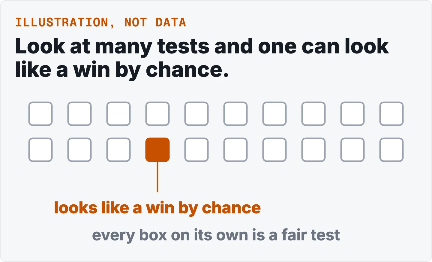
Run many tests and some will look like wins by chance. A correction keeps the chance of being fooled where you said it would be.
Run many tests at the 0.05 level and some will look significant by chance alone. The more tests you run, the more likely it is that at least one of them does [1][2]. That is the multiple comparisons problem. A correction changes the bar each result has to clear, so that the chance of being fooled stays where you said it would be. Which correction to use depends on what a false positive, a false win, costs you: whether a single wrong call is expensive, or whether you can live with a few wrong calls among many right ones [1][3].
Have your own list of p-values? The free multiple comparisons tool runs Bonferroni, Holm and Benjamini-Hochberg side by side.
Also on this topic: the business version, on a wine tasting test and the version for analysts, on the Benjamini-Hochberg procedure.
The answer first: many tests find false wins
Run many tests and some will look like wins by chance alone [1] [2]. A correction raises the bar each result has to clear, so the chance of being fooled stays where you said it would be [1]. Which correction fits depends on what one wrong call costs you [1] [3].
What this means for you
- Count every test you run. The more tests, the more likely at least one looks like a win by chance [2].
- Fix the list of tests before you look. Tests added after you see results do not count as the same family [8] [9].
- Pick the error you care about. A strict rule guards against any false win. A looser one allows a small share of false wins among many right calls [1] [3].
- Do not stop a test the first time it looks significant. Peeking is another source of the same problem [11].
What the multiple comparisons problem is: why many tests find false wins
A false positive, or false win, is a result that looks like a real effect when there is none. Each test at the 0.05 level carries a 5 percent chance of one when nothing is going on [2]. Across many independent tests, the chance that none of them produces a false win is 0.95 multiplied by itself once per test. In symbols, the chance of no false win across m tests is (1 - 0.05)^m [2][4].
| Tests with no real effect | Chance of no false win | Chance of at least one |
|---|---|---|
| 5. | 0.77. | 0.23. |
| 10. | 0.60. | 0.40. |
| 20. | 0.36. | 0.64. |
| 100. | about 0.01. | about 0.99. |
Rows 5, 10 and 20 are from [4]. The row for 100 is from [2]. The right-hand column is one minus the middle column.
The count of false wins grows the same way. A study of 10,000 genes, none with a real effect, tested at a 0.05 cutoff expects 10,000 x 0.05 = 500 false positives [3]. The same multiplication gives about 5 for 100 tests.
One lecture puts it as a coin: toss it long enough, however biased it is against heads, and sooner or later you see heads [2]. The same notes describe a drug study that fails on the whole population and is then retested in men, women, children, students and so on. With 100 independent tests at 0.05, a "winning" subgroup is almost certain to appear by chance [2].
A cartoon makes the same point. Scientists test 20 colors of jelly bean for a link to acne. Only green clears p < 0.05. The headline announces green jelly beans cause acne with "95% confidence" [5].
A research poster went further. A scanner tested over 40,000 small regions of the brain separately. A dead Atlantic salmon shown social photographs appeared to show brain "activation". With a multiple comparisons correction, the activation disappeared [6].
The problem does not need many tests on paper. Gelman and Loken point out that if the details of an analysis depend on the data, a researcher who ran one reasonable analysis "could have done other analyses that were just as reasonable" had the data come out differently [7]. The comparisons you would have made count too.
FWER vs FDR: two ways to count mistakes
There are two common ways to keep false wins in check. They answer different questions.
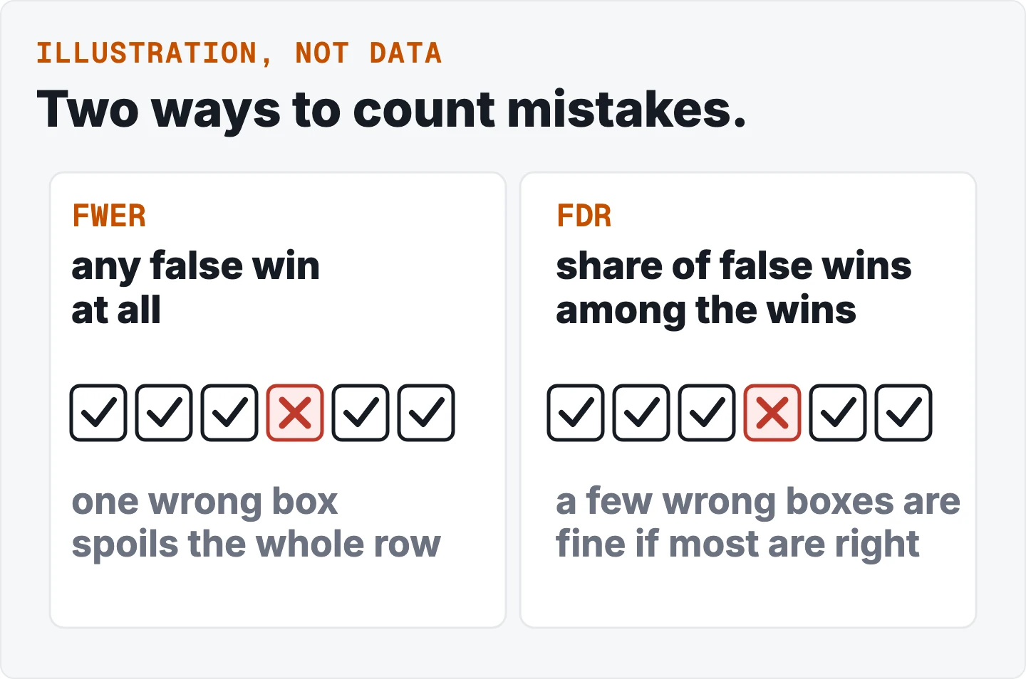
The family-wise error rate (FWER) is the chance of making any false win at all across the family [2]. Controlling it at 0.05 means the probability of even one false positive is under 0.05 [3].
The false discovery rate (FDR) is the expected share of false wins among the results you declare as wins [1][3]. If 550 of 10,000 genes are declared significant at an FDR of 0.05, the 5 percent is a long-run average share of declared wins, so on a list of 550 it points to roughly 27 false ones as a rough scale, but the count in any one list can be higher or lower [3]. When each hypothesis is in fact null, the FDR equals the FWER; otherwise it is smaller, so controlling it can find more real effects [1].
The business version. One A/B testing product notes that a 10 percent false positive rate can still mean a 50 percent false discovery rate when you declare two winners. One of the two may be wrong [12].
Which one fits depends on the cost of a wrong call. FWER suits work where any false positive is costly [3]. FDR suits exploratory work where "we can live with a certain number of false positives" [3]. An A/B testing blog gives the same split. The strict family-wise kind when false positives have serious consequences or you have few tests, the FDR kind for exploration across many segments or KPIs [13].
What counts as one family
A family is the set of comparisons you consider together [1]. For a Bonferroni correction it must be a finite set chosen in advance [8]. Running pairwise comparisons over and over for all pairs, as they occur to you, "will not, in general, work", because the overall error rate then differs from the one you specified [9].
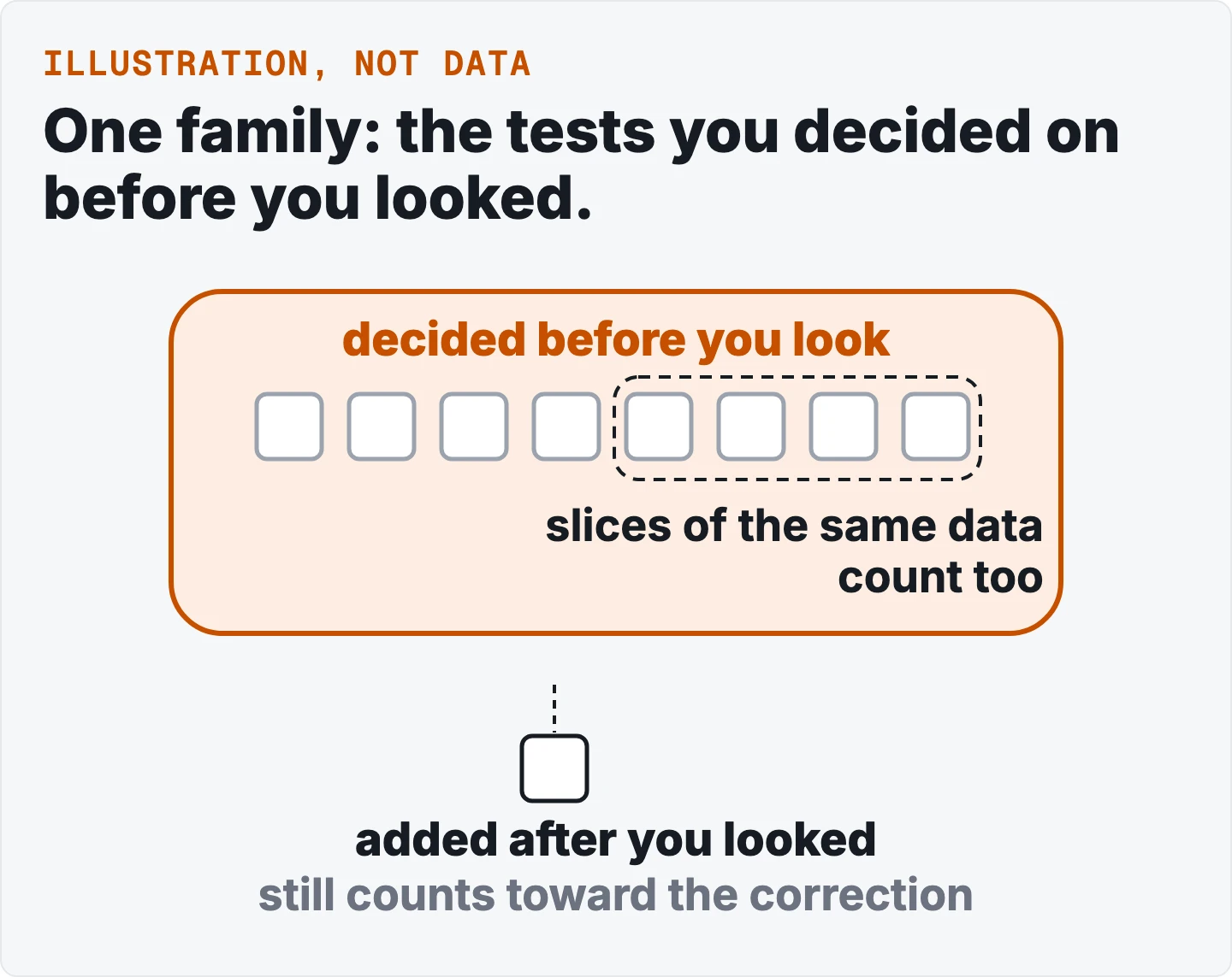
Products draw the line in different places. In one A/B testing product, the goal metrics across all variations form one family, and slices of the results by a dimension are corrected as a separate family. Its example: 2 variations x 4 goal metrics x a 3-level dimension gives 24 tests [10]. Segments multiply the count fast.
Peeking at a running test is a separate source of the same problem. In one essay's design, with no real effect, a test stopped the first time it looks significant at 5 percent, or after 150 observations, reaches a worst-case false positive rate of 26.1 percent against a nominal 5 percent [11]. To hold a real 5 percent, the same essay lists thresholds of 2.9 percent for one peek, 2.2 for two, 1.8 for three, 1.4 for five and 1.0 for ten [11]. Its remedy is to fix the sample size in advance [11].
Correction for multiple comparisons: which procedure fits
| Procedure | Controls | Assumption | Strength | What goes wrong |
|---|---|---|---|---|
| Bonferroni. | FWER. | A finite set chosen in advance [8]; valid for any dependence [2] | Simplest: reject when p is at or below 0.05 divided by the number of tests [2] | Often too conservative for many tests or dependent tests, which costs real effects [2] |
| Holm. | FWER. | Valid under any dependence [14] | Step-down: test the smallest p against the strictest bar, then relax the bar one step at a time [15][3]. More power than Bonferroni [3] | FWER methods can undermine power when the family is large [10] |
| Hochberg. | FWER. | Independent or non-negatively associated tests [14] | Step-up, derived as sharper than Holm [15] | Needs the dependence condition [14] |
| Benjamini-Hochberg. | FDR. | Proved for independent tests [1]; also holds under positive dependence [16] | Rank the p-values; find the largest rank j with p at or below (j / m) x 0.05; declare ranks 1 to j [3] | Does not bound the chance of any false win [3] |
| Benjamini-Yekutieli. | FDR. | Any dependence [16] | A rescaled version of the Benjamini-Hochberg step-up rule [16] | More conservative than Benjamini-Hochberg, and for small p-values can be more conservative than Bonferroni [14] |
The Bonferroni guide · The Holm guide · The Benjamini-Hochberg guide
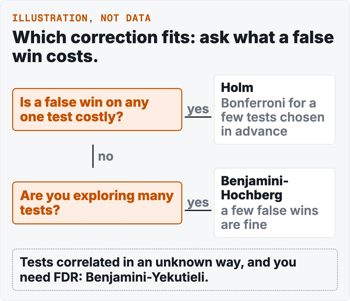
Two things follow from the table. If any single false win is expensive, use an FWER method. The R documentation sees "no reason to use the unmodified Bonferroni correction" because Holm is always at least as powerful [14]. Bonferroni still has a place when only a few comparisons, chosen in advance, matter [8]. If you are exploring many metrics or segments and can live with a few false wins, an FDR method finds more [14]. No single method of multiple comparisons is uniformly best [8].
What goes wrong in practice
Each correction costs power. Stricter corrections come "at the cost of lower power" [13]. One product warns that "with enough tests, controlling the FWER may completely undermine your test power" [10]. In one vendor's own analysis, Holm (with Hommel) gained about 4.5 points of ship rate over Bonferroni and Benjamini-Hochberg about 4.9, with the gap shrinking when few metrics have real effects [17]. The same vendor reports that two success metrics under Bonferroni raise the required sample size by roughly 20 percent [17].
The family you choose sets that cost. The same vendor says limiting the family to success metrics roughly halves the power cost for its median experiment, and that a partial correction is worse than none [17]. Products differ on guardrail metrics: that vendor leaves them out of the family [17], while another treats primary, secondary and monitoring metrics differently [12]. There is no single rule here.
Correlated tests change the arithmetic. Bonferroni is conservative when tests move together [2]. Benjamini-Hochberg holds under positive dependence; Benjamini-Yekutieli covers any dependence at the price of fewer wins [16]. Benjamini-Hochberg also assumes all p-values are in hand at one time, which does not fit tests read as they run [18].
Correct for the tests you ran, not only the ones you kept. In R, the count of comparisons is an argument of its own. The documentation spells out what it assumes about p-values you did not pass in [14]. Dropping the dull results before correcting makes the bar too easy.
In one product, adjusted p-values have no matching 95% range. An adjusted p-value can equal 1 [10]. Correcting the choice but not the estimate also inflates the effects you ship, a winner's curse [17].
Three questions tell you whether to trust a result picked from many. Was the family fixed before you looked? Is the error rate you controlled the one you care about? Did you correct for everything you ran?
How to run one on your own data
- List every test in the family, once each, before you look at the results.
- Pick the error rate you care about. Strict, for any false win. Or looser, for a share of false wins among your wins [3].
- Collect the raw p-values. Use them as computed, not rounded.
- Run the correction that fits and see which tests still win.
- Report the whole family, not only the tests that survived.
Try it on your own list of p-values with the free multiple comparisons tool.
What you need and what you get back
What your file needs: one row per test, and a column of raw p-values between 0 and 1. A test label column is optional. Use at least 5 tests. With fewer than 10, the corrections change little.
What you get back (these are facts about our tool, not general rules): Bonferroni, Holm and Benjamini-Hochberg side by side. You see which tests survive each one, the adjusted p-values, and the R code. The tool is free on up to 10,000 rows. Larger files are randomly sampled, and the report says so.
How we checked it
Three things to know about how this page was written.
Every claim has a source or a label
Each statement is tagged to the numbered reference it came from, or marked as ours. Our own framing is not presented as a sourced rule.
Our tool is described as ours
What the free tool needs and returns is stated as facts about our tool, not as rules from a source.
No numbers from a dataset
This page runs no data of its own. Its figures come from the cited sources and from arithmetic shown on the page, and the business and analyst articles show the idea on real data.
Questions people ask
Why does testing many things give false positives?
Each test at the 0.05 level has a 5 percent chance of a false positive when there is no real effect. Run many independent tests and those chances add up. The chance of at least one false positive is one minus 0.95 raised to the number of tests. At 100 tests it is about 0.99, so a false win is close to certain unless you correct for it [2].
Should I use Holm or Bonferroni?
Holm, in almost each case. Both control the chance of any false win across the family, but Holm tests the smallest p-value against the strictest bar and then relaxes it step by step, which gives it more power [3]. The R documentation says Bonferroni is dominated by Holm. There is "no reason to use the unmodified Bonferroni correction" [14].
Should I use Benjamini-Hochberg or Bonferroni?
It depends on the mistake you care about. Bonferroni controls the chance of any false win at all. Benjamini-Hochberg controls the expected share of false wins among the results you declare, which is a less strict target. It is typically more powerful [14]. Use Bonferroni-style control when one wrong call is costly, and Benjamini-Hochberg when exploring many metrics [3].
When do I need to correct?
Whenever you report a significant result picked from many comparisons. One A/B testing blog lists the usual sources: several KPIs, several segments, and peeking at results while the test runs [13]. Picking significant results out of many comparisons without a correction gives a "greatly increased false positive (significance) rate" [1].
How many tests count?
Each comparison in the family you decided on before looking at the data [8]. In one A/B testing product, goal metrics across all variations form the family, and breakdowns by a dimension are corrected as a separate family: 2 variations, 4 goal metrics and a 3-level dimension already make 24 tests [10]. Segments multiply the count quickly.
What if my tests are correlated?
Bonferroni stays valid but becomes conservative when tests move together. It misses real effects [2]. Benjamini-Hochberg holds for independent tests and under positive dependence. When the dependence is unknown and you need false discovery rate control, Benjamini-Yekutieli covers any dependence, at the price of declaring fewer wins [16].
Does peeking at results count?
Yes, and it is a separate problem from testing many metrics. With no real effect, a test stopped the first time it looks significant at 5 percent, or after 150 observations, can reach a false positive rate of 26.1 percent against a nominal 5 percent in the worst case [11]. The remedy is to fix the sample size in advance [11].
References
- Benjamini, Y. and Hochberg, Y. (1995). Controlling the False Discovery Rate: a Practical and Powerful Approach to Multiple Testing. Journal of the Royal Statistical Society B 57(1), 289-300
- Zuev, K. M. (2016). Statistical Inference, lecture notes including multiple testing. arXiv:1603.04929
- Iruczinski, I. Multiple comparisons, lecture notes. Johns Hopkins Bloomberg School of Public Health, Biostatistics
- NTNU. ST1201, Week 13 module
- Munroe, R. xkcd 882, "Significant". A cartoon
- Discover Magazine. fMRI gets slap in the face with a dead fish, on the poster by Bennett and colleagues (2009)
- Gelman, A. and Loken, E. (2013). The garden of forking paths
- NIST/SEMATECH e-Handbook of Statistical Methods, 7.4.7.3 Bonferroni's method
- NIST/SEMATECH e-Handbook of Statistical Methods, 7.4.7 How can we make multiple comparisons?
- GrowthBook. Multiple testing corrections. Product documentation, read October 2026
- Miller, E. How Not To Run an A/B Test
- Optimizely. False discovery rate control. Product documentation, read October 2026
- Statsig. Multiple comparison corrections in A/B testing. Vendor blog, read October 2026
- R documentation. p.adjust: Adjust P-values for Multiple Comparisons
- Hochberg, Y. (1988). A Sharper Bonferroni Procedure for Multiple Tests of Significance. Biometrika 75(4), 800-802. Restates Holm's step-down rule
- Döhler, S. (2016). A Discrete Modification of the Benjamini-Yekutieli Procedure. arXiv:1612.04838. Cited for its description of Benjamini, Y. and Yekutieli, D. (2001), The control of the false discovery rate in multiple testing under dependency, Annals of Statistics 29(4), 1165-1188
- Spotify. Confidence: multiple testing. Product documentation, read October 2026
- Robertson, D. S., Wason, J. M. S. and Ramdas, A. (2023). Online multiple hypothesis testing. Statistical Science 38(4), 557-575